The 1 Billion Row Challenge is a test of pure processing throughput, measuring how fast you can read 1 billion rows from a text file and compute the min, max, and mean for each of up to 10,000 weather stations. The problem is very open-ended and leaves plenty of room for optimization along the way. I first caught wind of this challenge about 2 years ago, but I wanted to wait until I was better equipped to take it on. Submissions have since closed, so I tested this against my own hardware: an Intel Core i5-10400 processor (6 cores, 12 threads, 2.9 GHz, 4.3GHz boost frequency), 16 GB of dual-channel DDR4 DRAM, rated for 3200 MHz, but limited to 2666 MHz since that's the speed officially supported by the processor. The official entries were evaluated on a Hetzner AX161, a 32-core machine with 128 GB of RAM. That machine holds the entire input (14.29 GiB, or 15.34 GB) in page cache several times over, whereas mine has less regularly available RAM than the file has bytes. Since I'm bottlenecked by I/O on this setup, I did most of my testing and profiling against a smaller file of 270 million rows, roughly a quarter of the full input. Below is the problem statement in case you aren't familiar.
Preface
One thing that I failed to consider before beginning this project is how big of
a role the page cache would play. In retrospect, it makes complete sense —those
pages that are fetched from disk are stored in RAM to prevent future accesses
from hitting disk. The biggest concept that I initially didn't understand was
that the page cache scales dynamically and can grow to fill almost all of the
physical RAM that isn't used by other processes. However, one look at the
available memory that I actually had using free revealed that I had much less
memory to work with than I initially anticipated: 15 GiB total, with only 14 GiB
of that actually being available on an idle machine, against an input file of
14.29 GiB (15.34 GB). There's no possible way for the entire file to be present
in the page cache, even without other processes running. During my initial
tests, as RAM filled up, any pages fetched from disk had to evict other clean
pages, even those that were read ahead by the kernel and had yet to be accessed,
requiring another major fault (trip to disk) when those pages are needed.
I did consider walking behind the scan with madvise(MADV_DONTNEED) to release
what I had already read, but that only tears down my own page table entries and
leaves the page cache pages resident.
Due to this, I decided to use a file with 270 million rows instead (3.86 GiB). Still a lot of data to parse, but small enough to stay resident in the page cache. This means that a warm run takes zero major faults and the challenge becomes a sheer measure of parse speed.
Naive Approach
My initial "naive" approach was deliberately unsophisticated. It followed a blueprint that remained mostly constant throughout my revisions — what changed over time was how each step was carried out, not the steps themselves.
This iteration was multithreaded, splitting the file into one roughly equal range of bytes per thread while ensuring that no row straddled a chunk. One approach that I considered but never attempted was handing out work dynamically to the threads. I believed that the coordination overhead would be too great and, in theory, each thread should finish around the same time anyway. Below is a brief outline of how each thread operated in this inital implementation. Consider how each of the underlined phrases might be changed / improved upon in future iterations:
- The thread processes one line at a time, finding the
delimiter with
std::ranges::findandstd::unreachable_sentinel, since the semicolon is guaranteed to appear on each line. - Parse the station and the temperature, storing the temperature as a 16-bit
integer, that value being . Add each
reading to a single, global
std::mapguarded by a global mutex, since every thread writes into the same table. - Track the running min and max with
std::min/std::maxalongside the sum and count for each station. - Once every thread joins, walk the table in sorted order and write each station's results to the output file.
On the smaller file, this took just under three minutes which isn't great. The
wall clock isn't necessarily the most interesting metric, however: the program
boasted a measly 0.53 instructions per cycle when we should be shooting for 2 or
more at least. perf revealed that my implementation spent more than 6x as long
inside the kernel (system time) as it did running its own code (user time). With
the file already warm in page cache, almost none of that system time is I/O, it
is the futex waiting. Every thread that loses the lock parks itself in a futex
wait, and every handoff back costs a trip through the scheduler. 270 million map
updates behind one lock means 270 million opportunities for a thread to block,
and the twelve threads I have available on my machine spent most of their time
doing exactly that, as seen by the 174 million context switches, at an effective
clock of 1.94 GHz. Nothing about the parse loop mattered yet.
Optimization 1: Poor Man's Map
I think that the most glaring issue with the naive approach is the use of a single source of state, protected by a mutex that twelve threads fight over. A much better approach comes from noticing that none of that state needs to be shared while the file is being read. The min and max computations are associative in nature, and the mean across all readings for a station can be extrapolated from the sum of its temperatures and the total number of readings, both of which are associative too. This means that every thread can keep its own table, keyed by station name, accumulating those four values as it processes its own chunk of the file. The twelve tables can be merged once the last thread has joined, removing the need for any synchronization between threads while the file is being read.
The tradeoff with this approach is that we are trading memory for speed, since
the table now exists twelve times over. My first iteration reached for the
obvious container for this, std::map:
struct Stats {
  int16_t min, max;
  uint32_t count;
  int64_t sum;
};

std::map<std::string, Stats> table;
std::map is the most natural choice for a container here, sorting the keys by
default, which is required for the final output. Merging the tables at the end
is cheap as well, since each thread's table holds at most 10,000 entries, so
folding all twelve into one costs at most 120,000 updates. The catch is that
each of the 270 million upserts completed while reading the file has to locate
its key by descending the tree, and the tree is only shaped that way to give me
an ordering I need exactly once, after the merge, to write 10,000 lines.
Inspired by this talk, we can do some napkin math to approximate how much space we'll actually use with this approach:
-
Each node is 32 bytes, 24 bytes for left, right, and parent pointers, 4 bytes for a red/black color field (defined as an unscoped enum), and 4 bytes of padding.
-
The string key is another 32 bytes per node.
-
The struct used to keep track of the stats for each station is 16 bytes, as seen in the above sample.
Note that the sum of the temperature readings needs to be 64-bits in the worst case where every reading is 99.9 at the same station. All 270 million rows landing on one station sums to approximately , which is greater than the maximum value of a
uint32_t, .
One thing to note is that every node creation calls its own operator new, and
glibc's allocator
prepends an 8-byte header and rounds the result up to a 16-byte boundary, so an
80-byte request occupies a 96-byte chunk. So, this means that, across all
threads, the maps allocate
Eleven megabytes against 16 GB of RAM sounds like a small price to pay, however, it is important to note that my machine only has 12 MiB of L3 cache that is shared across all six cores. The twelve maps fill 92% of L3 without counting a single byte of the input. Moving one level up and considering the L2 cache, it's worse still: two threads share a core's 256 KiB L2 between two ~940 KiB trees, so in practice every lookup misses L2.
If the requested value for a lookup is not in cache, odds are there will be more than one cache miss as we descend the map. A red-black tree with 10,000 nodes is, in the worst case, levels deep, so an access could pointer-chase all 26 nodes the allocator placed wherever it pleased into cache. This isn't to mention the string comparisons at every level that only make the operation costlier. 26 trips to L3 on each of 270 million upserts is unacceptable.
The obvious response is to swap in std::unordered_map and stop paying for
ordering we don't need. However, I found that it barely helped, and I believe
this is mostly due to the fact that it is still a node-based container that uses
buckets to handle hash collisions. Determining the bucket index of an item
relies on the division operation when the number of buckets isn't a power of two.
Instead of pursuing a node-based structure for our key-value store, we can write a much simpler table that lies contiguously in memory and avoids unnecessary overhead guaranteed by the standard: a fixed-size array of slots, indexed by a hash of the station name.
struct alignas(32) Slot {
  char name[16]; // 15 bytes + null terminator
  int16_t min, max;
  uint32_t count;
  int64_t sum;
};

// one per thread, 32K slots for at most 10,000 stations
std::vector<Slot> table(1u << 15);
By reserving space for the vector upfront, we bypass the need to request extra
memory on every insert. A power-of-two capacity allows us to map a hash to a
slot using the bitwise and operation instead of division via
hash & (capacity - 1).
With 10,000 stations in 32,768 slots, our load factor is . Using standard linear probing, finding a key that is already present takes approximately probes. Those extra probes are nearly free, though, since every slot is 32 bytes and aligned, so two slots share a cache line and spatial locality means the next slot is usually already present.
Continuing on the idea of napkin math, we see how the two structures compare per station entry:
Note that the poor man's map actually reserves more memory than the trees, since over two-thirds of its slots sit empty. But, this means that a lookup only ever touches, in the average case, the one or two slots its hash points to.
Now, with this new map, what was 26 dependent loads in the worst case collapse into one or two, and the address of that load is known the moment the hash lands, so the core can keep several rows' lookups in flight instead of stalling on each one in turn.
Running this against the same 270 million row input:
One detail that I glanced over was the hash function that I opted to use: a 64-bit fnv1a hash, which XORs each character of the station name into a 64-bit accumulator and multiplies by a prime. My initial implementation resembled the following code snippet:
static constexpr uint64_t hash(std::string_view sv) {
  uint64_t h = 14695981039346656037ull;
  for (unsigned char c : sv) {
    h ^= c;
    h *= 1099511628211ull;
  }
  h ^= h >> 32; // avalanche

  return h;
}
Note that the above constants are the "fnv1a" prime and offset basis, which abide by some constraints that I do not understand myself. Also, it is worth noting that the avalanche step at the end mixes the high bits down into the low ones I index with. The important thing to note from this snippet is that we must process each character in the station name serially, since each calculation depends on the value from the previous. To bypass this, we can use the fact that station names are bytes, allowing us to store the ASCII values of the characters in two 64-bit integers. Now, the number of operations needed to compute a hash stops growing with the size of the key: a three character station name now costs the same to hash as a fifteen character one. I also opted to use a fmix64 hash, based off of murmurhash, to compute the hash in three multiplications and three shifts:
static constexpr uint64_t hash(uint64_t s0, uint64_t s1) {
  uint64_t h = s0 ^ (s1 * 1099511628211ull);
  h ^= h >> 33;
  h *= 0xff51afd7ed558ccdull;
  h ^= h >> 33;
  h *= 0xc4ceb9fe1a85ec53ull;
  h ^= h >> 33;
  return h;
}
Both integers are loaded straight out of the mapped file with a pair of 8-byte
memcpy calls, then masked down to just the station name. We read all 16 bytes
regardless of how long the name is, but we can mask any bytes that run past the
name if we know the position of the delimiter that follows it (more on
optimizing this later). Reading only as many bytes as the name actually occupies
would mean either branching on the length or handing memcpy a runtime size,
which it can no longer fold into a pair of loads (for more on this, read
here).
Reading the maximum costs two and instructions instead, and since every name
is followed by a delimiter and a reading, the bytes we overshoot into are still
part of the same line. Note that the 9 possible bytemasks can be computed at
compile time, one for each number of bytes (0 through 8) the name can occupy in
either integer.
Putting the fixed-size keys, the compile-time masks, and the new hash function together, we get another great performance improvement over the previous iteration:
The instruction count fell from 65 billion to 36 billion and instructions per cycle rose from 0.66 to 0.88, so we're doing less work and stalling less often while we do it.
Optimization 2: SIMD / SWAR
Going back to the naive approach, each thread found the delimiters on a line
with std::ranges::find, which walks the line one byte at a time, comparing
each character against the delimiter and branching on the result. Branch
mispredicts can cost us a lot of clock cycles, so it is in our best interest to
remove them when possible. One look at perf report revealed that nearly 20% of
the program's clock cycles were spent within these searches, so it made sense to
turn to an alternative: SIMD. Most CPU cores come with a set of wide registers
that allow a single instruction to operate on several values at once, and the
i5-10400 on my workbench has sixteen 256-bit registers that support AVX2
instructions. Since a station name is at most 15 bytes, the name and the
semicolon that follows it always fit within the 32 bytes that one of these
registers holds. So, instead of checking one character at a time, we can load 32
bytes of the line into a register, compare every byte against a semicolon in a
single instruction, and reduce the result to a 32-bit mask whose lowest set bit
marks the position of the delimiter. The same trick finds the newline, and
neither search loops nor branches per character. In the best case, a single load
could find the delimiters of readings at a
time (more on this later).
A SIMD load from L1 usually takes between 5 and 7 cycles on AVX2, which is a small price to pay for the boost in processing throughput.
Running the AVX2 search against the same input:
Note that instructions per cycle actually fell from 0.88 to 0.64, which looks like undesired at first glance. However, the instruction count fell from 36 billion to 23 billion, so we're doing far less work overall. Branch mispredicts fell from 710 million to 196 million too, even though a larger percentage of branches now mispredict, since the total number of branches dropped from 11.6 billion to 1.7 billion. This solved part of the branch mispredict issue, but we are still mispredicting of all branches.
The remaining branch mispredicts are still the glaring issue, even after
improving our delimiter search. I had reason to believe, from more digging
through perf report, that most of them came from parsing the temperature,
which checks for a minus sign and for whether the reading has one or two digits
before the decimal point. Since the temperature readings in the input are
generated at random, I originally figured neither check could be predicted
reliably. The fix I found
here,
from another programmer attempting the same challenge, used SWAR (SIMD within a
register), which applies the same idea as SIMD to an ordinary 64-bit
general-purpose register. A reading is at most 6 bytes long (-99.9 and the
newline), so the entire reading fits into a single 8-byte load and its value can
be pulled out with some bit manipulation and a single multiplication, without
branching on the sign or the number of digits. I still don't understand fully
how this works; it is quite the feat. Credit to
merykitty, who pioneered the method.
The catch with this approach that doesn't pair well with the previous optimization is that SWAR lives in a general-purpose register, not the vector registers that we just used to find the delimiters. Parsing a number depends on where each of its digits sits, and each reading starts at a different offset within the register, so AVX2 provides no easy way to line them up in lanes and parse several at once. To solve this, we have the SIMD search only return the position of the semicolon, and the 8 bytes after it are loaded again into a general-purpose register to be parsed one reading at a time (if there is a clever way to work around this double load, please let me know). SWAR also finds the end of the line on its own, since the newline always sits two bytes after the decimal point, which makes the SIMD search for the newline redundant.
My implementation of the SWAR temperature parse can be found here. Running this new temperature parse against the same input:
Surprisingly, this change caused the program to run slower with the average wall
clock rising from 0.822 seconds to 0.855 seconds, even though branch mispredicts
fell from 196 million to 166 million. As it turns out, after digging through the
disassembly, there was a different root to the branch misprediction issue than I
originally expected: a single std::min call used to split the station name
across the two 8-byte integers had compiled to a branch. Since station names
vary randomly in length, that branch was responsible for the vast majority of
the remaining mispredicts. Here's how I originally stored the value of the
station name:
// RECALL: store the name in two 8-byte integers (name <= 15 bytes)
std::memcpy(&s0, begin, sizeof(uint64_t));
std::memcpy(&s1, begin + sizeof(uint64_t), sizeof(uint64_t));

// "branchless" store name (assumes little endian layout)
const size_t sep = std::min(station_length, size_t{8}); // compiles to a branch
s0 &= station_masks[sep];
s1 &= station_masks[station_length - sep];
This branch will likely be mispredicted on around half of the lines, assuming
the length of the station is truly random between 1 and 15 characters. This will
lead to around million pipeline flushes, costing around
20 cycles each (a rough estimate, which I check below). To get rid of this
branch, I replaced the 9 single masks with a lookup table of mask pairs, one for
each possible name length. The previous version had to compare the length
against the size of the integers where the names were stored (8 bytes) to decide
how the name splits across the two integers before it could look up either mask.
The new table bakes that split into every entry, so a single lookup by the full
length returns both masks and nothing compares against the length at all. Note
that the table in both versions is marked as constexpr and is evaluated at
compile time:
// one {low, high} mask pair per possible name length, built at compile time
// ex: station_masks[12] = {low_bytes: 255, high_bytes: 240}
const StationNameMask station_name_mask = station_masks[station_length];
s0 &= station_name_mask.low_bytes;
s1 &= station_name_mask.high_bytes;
Running this against the same input:
Branch mispredicts fell from 166 million to 32 million, which confirms that the
std::min was responsible for most of them, and only 2.77% of branches now
mispredict. The wall clock also fell to 0.796 seconds, beating the 0.822 seconds
from Table 4. Cycles fell by 2.5 billion as well, which puts each removed
mispredict at no more than about 18 cycles, in line with the estimate above.
As for why the SWAR parse made the program slower with fewer mispredicts, I believe it comes down to a control dependency versus a data dependency. A branch can be speculated past, in which case the digit check guesses correctly and incurs no cost. The digit check also would have been guessed correctly about 90% of the time, given 190 out of the 1990 possible temperature measurements have a single-digit integer part. On the other hand, a branchless computation can't be speculated past, so we never encounter a zero-cost digit check.
Optimization 3: Thread Count
Up until now, every run has used twelve threads, exactly what
std::thread::hardware_concurrency() reports. I thought that this would
maximize performance, falling for the "more threads implies greater throughput"
fallacy. However, the i5-10400 only has six physical cores, and hyperthreading
runs two threads on each one, with those two threads sharing execution units and
its L1 and L2 caches. What I failed to realize is how this would affect
performance, especially with threads fighting for cache space. To evaluate the
effect the number of threads had on the throughput of my program, I ran it with
all possible thread counts and compared the average runtimes across five warm
runs.
Sweeping from one to twelve threads:
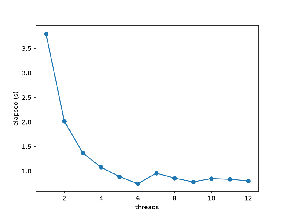
Wall clock vs. thread count, 270 million rows
The wall clock falls steadily up to six threads, bottoming out at 0.740 seconds, then jumping to 0.954 seconds at seven and not recovering the gains we got from six threads. Past six threads, each additional thread doubles up on a core, competing for its caches as well. Every thread keeps its own 1 MiB table. Six tables take up half of the 12 MiB L3, but twelve fill it entirely before a single byte of input is read. Sure enough, the LLC (last level cache) load misses stay flat at around 4.4 million up to six threads, then climb with every thread after that, reaching over 32 million at twelve:
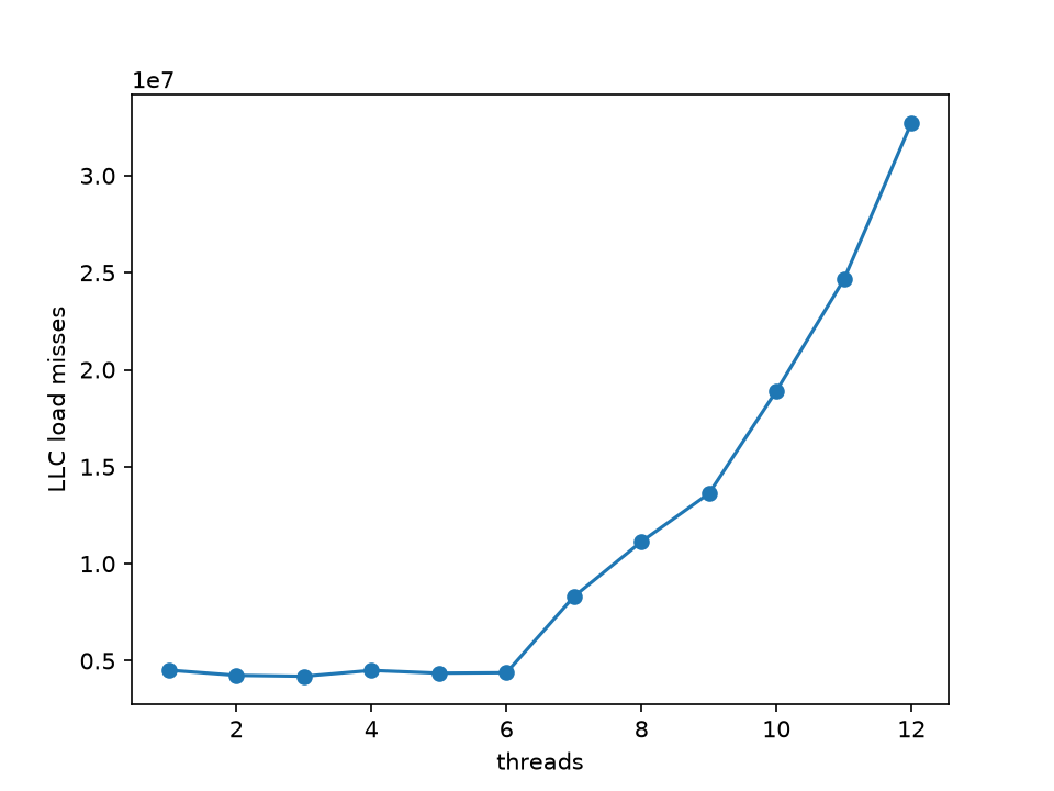
LLC load misses vs. thread count, 270 million rows
Setting the thread count to six, a one-line change, brought the wall clock from 0.796 seconds to 0.739 seconds, a 7.1% improvement. Instructions per cycle also jumped from 0.63 to 1.32.
Small Nits
I was pretty satisfied with the results up to this point; I had brought the runtime to under a second on a fairly dated, budget processor. However, I knew there was still some performance on the table. Finding what worked required lots of trial and error; below is a list of the small nits that won and lost me time. All of these were built and tested on top of my six-thread program, and I'll start with the ones that didn't work out. Assume that any mention of a map or a table refers to the Poor Man's Map I implemented per Optimization 1.
What Didn't Work
-
Decreasing Table Size: Halving the size of the table to 16,384 slots (from 32,768 slots) shrank each thread's table to 512 KiB, which nearly halved LLC load misses from 4.32 million to 2.27 million in my testing. However, the load factor doubled to , so a lookup took about 1.78 probes instead of 1.22. This was reflected in the number of branch mispredicts, which skyrocketed from 32 million to 82 million. This change increased my average wall clock time by 8.7%.
-
Buffering Writes (Instead of Batching): Upon completion of processing a chunk of the input file, each thread returns a map. The batching described below writes 32 lines back to the table at once, so only one iteration incurs the cost of the writes. I tried spreading that out with a ring buffer that writes back one line per iteration, amortizing, in theory, the work done by the batched write. However, this change added 3.9 billion instructions, and even with instructions per cycle rising from 2.15 to 2.40, it ran slower.
-
Disabling Source Fortification: It turns out that glibc provides protection against buffer overflows via a feature called source fortification, which some GCC builds enable by default. Since I load each station name as raw bytes from the mapped file with two
memcpycalls, I assumed each one carried a runtime bounds check, asmemcpyis one of the functions it hardens. However, building with-U_FORTIFY_SOURCE -D_FORTIFY_SOURCE=0didn't reduce the instruction count. Each copy is a constant 8 bytes into an 8-byte integer, so the compiler had already proven the bounds checks unnecessary. A 0.7% difference is the same as what I got from rebuilding identical code, so this one is noise.
What Worked
-
Scanning 64 Bytes at a Time: Instead of loading 32 bytes at the start of every line, I decided to load 64 bytes into two registers and find the delimiters via a 64-bit mask of every semicolon and newline.
std::countr_zerogives the position of the next delimiter andx &= x - 1clears it, so one window covers every complete line inside it, up to 10 readings compared to one per load before. One thing that I didn't even consider until I looked into simdjson was the fact that this approach could technically read past the end of the file I mapped at the beginning of the program. The fix I borrowed from simdjson is to first map an anonymous region 64 bytes larger than the file, then map the file over the front of it. This ensures that the final window reads zeros instead of unmapped memory if it reads past the mapped boundary with a 64-byte access. This change by itself does not have a big impact on performance, but I think it is still worth touching on. These changes brought the wall clock down 6.6% on average. I believe this is because a line no longer had to wait on the previous line's newline position before it could load. Every delimiter in a window is known after the same two loads, so the work for the roughly four lines in each window could overlap. -
Prefetching and Batching Map Operations: When I profiled the program back in Optimization 1, about 30% of its cycles landed on a single load: reading a slot's key out of the table. So, instead of updating the table as soon as a line is parsed, I hash the name, prefetch its slot with
__builtin_prefetch, and park the line in a batch of up to 32. Once the batch is nearly full, I write it back, by which point its slots should already be in L1. This was by far the biggest win of the bunch, decreasing average runtime by 10.6%, with instructions per cycle rising from 1.61 to 2.15 even as the instruction count went up. -
Branchy Min / Max: A station's running min and max rarely change, since the number of new min / max values that will overwrite the previous min / max grows logarithmically with the number of readings. Logically, this makes sense: a new reading only replaces the min if it is lower than every reading before it, and that bar gets harder to clear the more readings we've seen. Because the readings are random, each of the first readings is equally likely to be the lowest, so the -th reading is a new minimum with probability . Over readings, we expect about new minimums and likewise for the max. That sum only grows by about each time doubles. Each thread sees about 4,500 readings per station, so its min and max are each expected to change fewer than 10 times.
std::min/std::maxcompiled tocmovs, which are paid on every reading. The solution is to replace these calls with plainifstatements. The real win here was marking both branches[[unlikely]], which moved the stores to the end of the function, so the common case falls straight through, bringing the wall clock down 3.2%. -
Multiply-Shift Hash: The fmix64 hash from Optimization 1 chains three multiplications, each of which has to wait on the result of the one before it. I replaced it with just two multiplications, one for each half of the station name, each by one of xxHash's primes. Neither depends on the other, so both can run at the same time. I then XOR the two products together and keep the top 15 bits as the slot index, since the high bits of a product are the best mixed. This reduced the instruction count by 2 billion and brought the wall clock down 5.2% on average.
-
Packing Count and Sum: Instead of storing the count and sum separately, the two can be packed into a single 64-bit integer, reserving 24 bits for the count and 40 for the sum. This allows each reading to update both values with a single RMW (read-modify-write) instead of two. This saved 1.1%, but the catch is that a 24-bit count overflows past 16.7 million readings for a single station. Luckily, this is far more than the roughly 27,000 each station sees here, though the problem statement technically allows it. Since each reading adds at most 999 tenths to the sum (I store the readings in tenths to avoid floating point numbers), a 24-bit count also keeps the sum below , so the sum only needs 35 bits, sign included. This means the split can be modified to suit how many readings each station will likely see: 26 bits for the count and 38 for the sum, for example, raises the limit to about 67 million.
-
Exiting Early: The final improvement I found is a cool one. My program originally called
munmapon the 3.86 GiB input file and closed the file before returning frommain, which also runs every destructor. Callingstd::_Exitskips themunmapand all of the stack unwinding for local and static variables, although the kernel still has to tear down the mapping when the process exits. In my testing, themunmaptook about 50 ms while the kernel's own teardown took about 45 ms, and that difference makes up most of the 1.3% improvement I saw in the average wall clock.
Final Results
In the end, the final throughput numbers are as follows:
I am proud of how this project went. My code can be found on my GitHub.