Particle Simulation: Improving Performance by 20x

Real-time particle simulation with 12,500 particles on a 2020 MacBook Pro (Apple M1, 8-core CPU, 8 GB RAM).

The world of physics and mathematics are greatly intertwined. It is very much a two-way relationship, where mathematical concepts can be used to describe physical phenomena, and physical experiments can lead to new mathematical insights. The goal of this project was to explore this relationship by creating a particle simulator, giving me the avenue to dive deeper with C++ optimization and object-oriented design in hopes of creating something that interests me as a software developer.

Verlet Integration

First, I think that it is important to discuss the physics behind the simulation. The particles in the simulation are influenced by gravity and also interact with each other through collisions. To model this effectively and simply, I chose to use Verlet Integration, as it provided a simple means of approximating the motion of particles in a way that is both efficient and easy to implement. Here's a cool derivation of the equations involved. Feel free to skip over the math if you're not interested.

Let’s start at the beginning. A particle’s motion is governed by Newton’s second law:

\begin{aligned} m\,\mathbf{x}''(t) &= \mathbf{F}(\mathbf{x}, t),\\ \mathbf{x}''(t) &= \mathbf{a}(\mathbf{x}, t) := \frac{\mathbf{F}(\mathbf{x}, t)}{m}. \end{aligned}

In my code, gravity is constant, so $\mathbf{a}(\mathbf{x}, t) = \langle 0,\, g \rangle$ .

Now expand the position about time $t$ using Taylor series. The general (one-dimensional) Taylor formula is

f(t+h) \;=\; f(t) + f'(t)\,h + \frac{f''(t)}{2!}\,h^{2} + \frac{f^{(3)}(t)}{3!}\,h^{3} + \cdots

Set $h=+\Delta t$ for a forward step:

\mathbf{x}(t+\Delta t) = \mathbf{x}(t) + \mathbf{v}(t)\,\Delta t + \tfrac{1}{2}\,\mathbf{a}(t)\,\Delta t^2 + \tfrac{1}{6}\,\mathbf{j}(t)\,\Delta t^3 + \mathcal{O}(\Delta t^4),

and set $h=-\Delta t$ for a backward step:

\mathbf{x}(t-\Delta t) = \mathbf{x}(t) - \mathbf{v}(t)\,\Delta t + \tfrac{1}{2}\,\mathbf{a}(t)\,\Delta t^2 - \tfrac{1}{6}\,\mathbf{j}(t)\,\Delta t^3 + \mathcal{O}(\Delta t^4),

where $\mathbf{v}=\mathbf{x}'$ is velocity and $\mathbf{j}=\mathbf{x}'''$ is jerk.

Adding these two expansions together eliminates the velocity and jerk terms:

\mathbf{x}(t+\Delta t) + \mathbf{x}(t-\Delta t) = 2\,\mathbf{x}(t) + \mathbf{a}(t)\,\Delta t^2 + \mathcal{O}(\Delta t^4).

Solve for the unknown future position gives us finally:

\boxed{\; \mathbf{x}(t+\Delta t) = 2\,\mathbf{x}(t) - \mathbf{x}(t-\Delta t) + \mathbf{a}(t)\,\Delta t^2 \;}

This gives us a formula only dependent on the current and previous positions of the particle (assuming constant acceleration), simplifying our calculations greatly. Here's an outline of how I calculated this for each particle in C++:

struct Vec2 {
  float x, y;
};
 
struct Particle {
  vec2 position;
  vec2 lastPosition;
  vec2 acceleration;
 
  void update(float timeDiff) {
    vec2 newPosition =
      2.0f * position - lastPosition + acceleration * (timeDiff * timeDiff);
    position = newPosition;
    lastPosition = position;
  }
};

Spatial Hash Grid

Next, let's discuss some of the design choices I made while implementing the simulator. Thinking broadly, noticing collisions between particles is something that seems trivial, but doing it efficiently can be complex. A naive approach would be to check every particle against every other particle, which is incredibly inefficient when you realize that there is no need to check for collisions between distant particles. Thus, to optimize this, I implemented a spatial hash grid, where each particle belongs to a specific cell in the grid, allowing for more efficient collision detection by limiting collision checks to only particles in surrounding cells.

struct Grid {
  std::vector<Cell> cells;
  struct Cell {
    std::vector<uint32_t> particleIndices;
 
    void addParticle(uint32_t idx) { particleIndices.push_back(idx); }
 
    bool removeParticle(uint32_t idx) {
      for (auto it = particleIndices.begin(); it != particleIndices.end();
           ++it) {
        if (*it != idx)
          continue;
        std::iter_swap(it, particleIndices.end() - 1);
        particleIndices.pop_back();
        return true;
      }
      return false;
    }
  };
};

Using this spatial hash grid approach, we go from iterating over all particle pairs to checking each cell and surrounding cells, which significantly reduces the number of checks needed as the number of particles grows. We can also tune the size of each cell as needed for maximum performance.

Collision Detection

On the collision side of things, handling them efficiently is key. Since square root is a costly operation in terms of performance, with a latency of up to 32 clock cycles on most ARM architectures, using this operation sparingly will be required. To do so, we can avoid it altogether by using squared distances instead of actual distances when checking for collisions. Concretely, given particles $p_1$ , $p_2$ with centers $c_1$ , $c_2$ and radii $r_1$ , $r_2$ , we can check for a collision by verifying if the squared distance between their centers is less than the squared sum of their radii:

\|\mathbf{c_1} - \mathbf{c_2}\|^2 < (r_1 + r_2)^2

\implies \sqrt{(c_1.x - c_2.x)^2 + (c_1.y - c_2.y)^2}^2 < (r_1 + r_2)^2

\implies (c_1.x - c_2.x)^2 + (c_1.y - c_2.y)^2 < (r_1 + r_2)^2

This calculation costs only a few multiplies and is great for when we’re solely concerned with whether or not the two particles are touching. Once we determine that two particles are indeed colliding, we need to resolve the collision by adjusting their positions and velocities accordingly. To do so, we can use the normal vector between the two particles' centers to determine the direction of the collision. This can be calculated as follows:

\mathbf{n} = \frac{\mathbf{c_1} - \mathbf{c_2}}{\|\mathbf{c_1} - \mathbf{c_2}\|} = \frac{\mathbf{c_1} - \mathbf{c_2}}{\sqrt{(c_1.x - c_2.x)^2 + (c_1.y - c_2.y)^2}}

We can then calculate the overlap to push each particle by half the overlap in opposite directions with respect to the normal vector calculated above. In C++, this can be implemented as follows:

#include "particle.hpp"
#include <cmath>
 
void solveCollision(Particle &p1, Particle &p2) {
  constexpr float epsilon = 1e-4;
  const float expectedDistance = static_cast<float>(p1.radius + p2.radius);
  vec2 axis = p1.position - p2.position;
  const float squaredDistance = axis.x * axis.x + axis.y * axis.y;
 
  if (squaredDistance < expectedDistance * expectedDistance &&
      squaredDistance > epsilon) {
    const float actualDistance = std::sqrt(squaredDistance);
    const float overlap = expectedDistance - actualDistance;
    const float delta = 0.5f * overlap;
 
    const vec2 colVec = (axis / actualDistance) * delta;
 
    p1.position += colVec;
    p2.position -= colVec;
  }
}

Now, we only use the square root operation when necessary and handle collisions correctly.

With all of this in place, I was able to achieve a real-time simulation with around 750 particles running at 60 FPS before hitting the performance limits of my hardware. This is a far way from achieving my goal of 15,000 particles, but it’s a promising start. Now, let's look at the optimizations that I made to improve performance and scalability.

Improved Collision Checking

The first big improvement that saw a ~2x increase in performance was optimizing the collision detection algorithm by reducing unnecessary cell-neighbor checks. Instead of checking all 8 neighboring cells and the current cell for potential collisions, it turns out that we only need to check 4 of the 8 surrounding cells. To illustrate this, consider the following diagram.

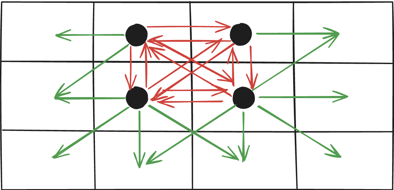
Naive neighborhood with duplicate checks.

Here, notice that we are checking all of the neighbors, redundantly pairing the same two cells multiple times for the four cells that we are concerned with. For many cells, this results in unnecessary computations. For an optimized approach, we can simply check only the cells below and to the right. Consider this diagram of our improved cross-cell checking:

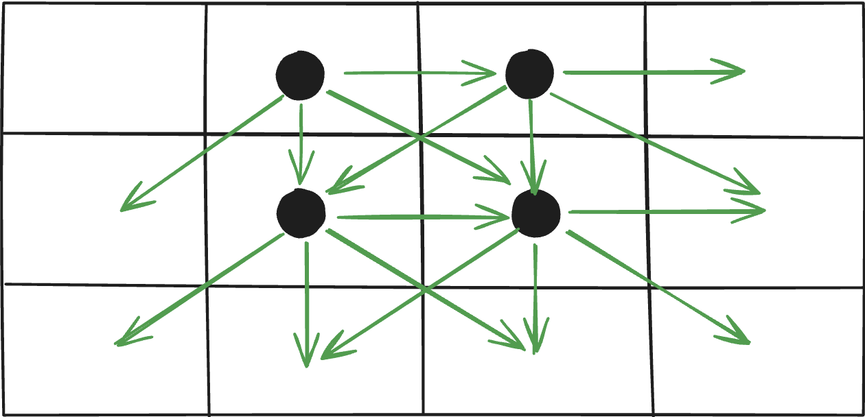
Half-stencil check without duplicates

With this improvement, we reduced our collision checking workload by half, leading to a ~2x performance gain, all while maintaining accurate collision detection. This moved our total particle count from 750 to 1500 while still achieving 60 FPS.

Sparse-Row Pruning

On a similar note, one problem that I ran into was a performance bottleneck regarding grid cell checks, similar to the one described above. Scanning every cell every frame is just too expensive. Profiling with sample showed the hotspot clearly:

Analysis of sampling ParticleSim (pid 57601) every 1 millisecond
Process:         ParticleSim [57601]
----

Call graph:
    12770 Thread_5418255: Main Thread   DispatchQueue_<multiple>
    + 12770 start  (in dyld) + 2840  [0x198368274]
    +   9483 main  (in ParticleSim) + 600  [0x10454174c]
    +   ! 9128 PhysicsEngine::update(float)  (in ParticleSim) + 132  [0x104541a5c]
    +   ! : 9007 PhysicsEngine::checkAllCollisions()  (in ParticleSim) + 112  [0x104549480]
    +   ! : | 4318 PhysicsEngine::processNeighboringCells(int, int)  (in ParticleSim) + 552  [0x104549d38]
    ...
    +   ! : | 1934 PhysicsEngine::processNeighboringCells(int, int)  (in ParticleSim) + 572,388,...  [0x104549d4c,0x104549c94,...]
    +   ! : | 734 PhysicsEngine::processNeighboringCells(int, int)  (in ParticleSim) + 388  [0x104549c94]

Notice how over half of the frames in the simulation were spent checking grid neighbors, some of which had no particles present. To address this, we can implement a active-row pruning technique. The idea is to keep track of which rows contain particles and only check those rows during each iteration. This significantly reduces the number of cells we need to check, leading to further performance improvements. Within the spatial hash grid, we can maintain the following: a flag for if the row has any particles at all, a count of how many non-empty cells live in that row, and the tight inclusive span $[\text{rowMinCol}, \text{rowMaxCol}]$ that brackets the first and last non-empty cell. Every frame, these values are updated incrementally as particles move. This is how I implemented this for when a particle is inserted into and removed from a cell:

Per-row state to maintain (updated as particles move):
  - rowHasActive[r]: whether row r has any non-empty cells.
  - rowNonEmptyCount[r]: number of non-empty cells in row r.
  - rowMinCol[r], rowMaxCol[r]:
      tight inclusive span of non-empty columns in row r.
 
# When inserting a particle at cell (r, c)
insert:
  - add particle id to Cell(r, c)
  - increment rowNonEmptyCount[r]
  - if cell was empty before:
      rowHasActive[r]: true
      rowMinCol[r]: c
      rowMaxCol[r]: c
    else:
      rowMinCol[r]: min(rowMinCol[r], c)
      rowMaxCol[r]: max(rowMaxCol[r], c)
 
# When removing a particle from cell (r, c)
remove:
  - remove id from Cell(r, c) via swap-and-pop
  - decrement rowNonEmptyCount[r]
  - if cell became empty:
      rowHasActive[r]: false
      rowMinCol[r]: +INF
      rowMaxCol[r]: -1
    else:
      if c == rowMinCol[r]: RecomputeRowMin(r, start=c+1)
      if c == rowMaxCol[r]: RecomputeRowMax(r, start=c-1)

Mathematically, this changes the number of cells that we consider each frame from

\Theta{(N)}

\Theta{\left(\Sigma_{r \in \text{active rows}} (rowMaxCol[r] - rowMinCol[r] + 1)\right)} = \Theta{(M)}

where $M \leq N$ is the number of non-empty cells in the active rows. This optimization yielded another ~2x performance improvement, allowing us to reach a total of 3000 particles at 60 FPS.

Parallelizing Collision Detection

In my opinion, this is the coolest optimization of them all. It took real design work, and I’m happy with where it landed. The core is a single shared MPMC (multi-producer, multi-consumer) work queue protected by a mutex and a condition variable. Any thread can push; any thread can take. Pushing a task increments an atomic in-flight counter and signals the condition variable so sleeping consumers wake promptly. After a task finishes, the in-flight counter is decremented and the condition variable is signaled again, so waiters observe progress immediately. The queue keeps a closed bit as well: once set, consumers wake, drain any remaining tasks, and then exit cleanly when the queue becomes empty. The invariant here is that a frame is considered “done” exactly when the work queue is empty AND the in-flight counter is zero. That definition is cheap to test and doesn’t require per-task joins.

On top of that queue, a fixed-size thread pool runs a set of worker threads. Each worker loops: sleep when there’s no work, wake on push/close, run a task, account for completion, repeat. Because idling uses the condition variable, there’s no busy-waiting; idle cores truly go idle. The main loop submits a batch of coarse tasks for the current frame (e.g., bands of grid rows), then waits for completion using the same queue semantics. While waiting, it cooperatively drains the queue via the non-blocking path—if a task is available, it runs it immediately; if not, and work is still in flight, it parks on the condition variable and wakes on progress. This shortens the tail of each batch and keeps frame pacing tight without introducing a second synchronization primitive.

A few implementation details that matter for throughput and correctness:

Exception safety. Task execution is wrapped so the in-flight decrement always happens (even if a task throws), keeping the “done” predicate accurate.
Fairness. The queue is FIFO at the push/pop level; the main thread is just another consumer—there’s no special priority, only cooperative draining.
Close semantics. Closing doesn’t discard pending work; consumers continue popping until empty, then observe closed + empty and exit.
Coarse tasks. Submitting row-band jobs (instead of thousands of per-cell jobs) reduces queue contention, improves cache locality, and limits scheduling overhead; combined with the half-stencil grid checks and two-stripe passes, no two tasks write the same particles in a pass, so the collision phase remains lock-free.

Aside - Wavefront Scheduling: I didn't see any significant improvement in performance with multithreading until I changed what each task looked like. This involved giving each worker a contiguous band of rows (e.g., 2–8 rows) and processing them left-to-right. Then do a second pass offset by one row so cross-row pairs that straddle band boundaries are covered without duplication. In practice this looks like two stripes: pass A handles rows $[a, a + 2, \cdots, a + 2k - 2]$ ; pass B handles $[a + 1, a + 3, \cdots, a + 2k - 1]$ ; Each band is one coarse task. This led to fewer tasks in the queue compared to each cell being its own task and removing the need for locks within each cell since there is no possibility of cross-cell interference using the two-stripe approach.

#include <algorithm>
#include <vector>
 
void collideWavefront(uint32_t rowsPerTask = 4) {
  const uint32_t R = collisionGrid.rows, C = collisionGrid.cols;
  rowsPerTask = std::max<uint32_t>(1, rowsPerTask);
 
  auto submitStripe = [&](uint32_t startRow) {
    std::vector<std::pair<uint32_t, uint32_t>> bands;
    bands.reserve((R + rowsPerTask - 1) / rowsPerTask);
 
    for (uint32_t r0 = startRow; r0 < R; r0 += rowsPerTask) {
      const uint32_t r1 = std::min<uint32_t>(R - 1, r0 + rowsPerTask - 1);
      // optional: skip fully empty ranges if you maintain row headers per
      // optimization 2.
      // if (!bandHasWork(r0, r1)) continue;
      bands.emplace_back(r0, r1);
    }
    // one task per band
    for (auto [r0, r1] : bands) {
      pool.addTask([this, r0, r1, C] { processBand(r0, r1, C); });
    }
    pool.waitIdle(); // single barrier for this stripe
  };
  submitStripe(0); // rows [0, 2, ...]
  submitStripe(1); // rows [1, 3, ...]
}

After implementing this, I saw a ~1.5x performance improvement on my 8-core machine, allowing for simulations with 4500 particles to be run at consistent 60 FPS.

Flattening the Grid

The biggest single speedup came from reshaping the grid from a nested vector<vector<Cell>> to a single, flat row-major array vector<Cell>. This came as a big surprise to me, but makes sense when you consider memory access patterns. In the nested layout, every cell access does two pointer dereferences (row, then column), rows live in separate heap allocations, and traversal bounces around memory. This way, neighbors become fixed-offset indices in one contiguous buffer, leading to much better cache locality. This optimization led to the biggest improvement in performance, around 4x, allowing for up to 15000 randomly generated particles to be simulated at once.

I'm incredibly happy with what came out of this project. The source code is on available on GitHub. But, what's next? The goal is to extend this to fluid dynamics in the near future. Stay tuned for that.